3D Mesh Surface Reconstruction From Point Clouds
In this project, Reyhan Pamungkas and I attempt to recreate the solutions of the SMRVIS: Point cloud extraction from 3-D ultrasound for non-destructive testing Paper by Tang, L. T. W. for a challenge hosted by UBC Data Science Club in collaboration with DarkVision, a British Columbia-based company that specializes in industrial imaging technology. The code for this project can be found here.
Introduction to The Challenge
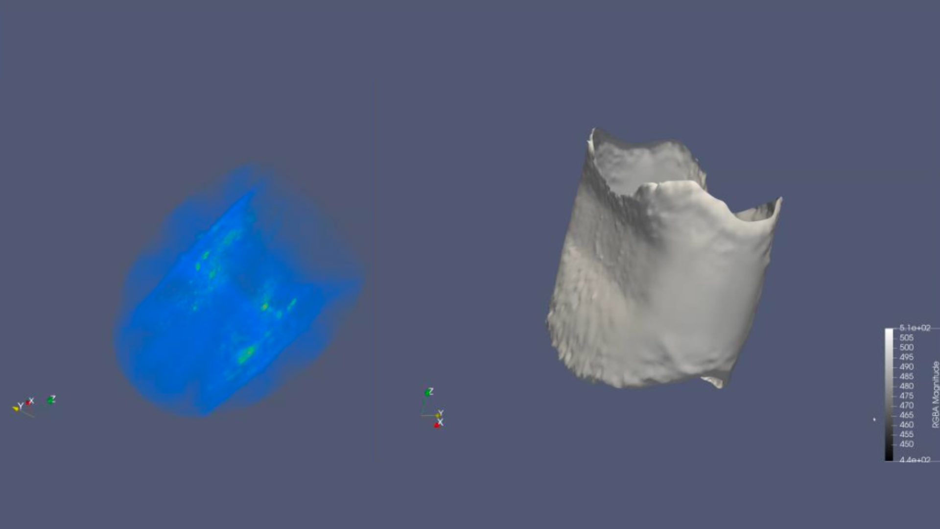
The techniques that this project used, was utilized in biomedical imaging such as CT and SPECT scans, but we repurpose it for non-destructive testing of industrial components, such as steel pipes. By detecting manufacturing defects in steel pipes, the framework has industrial applications in quality assurance and safety. The challenge didn't provide a definitive guide that told us to recreate the solutions of the SMRVIS Paper, not until 2 days after the challenge was published. Hence, the methodologies tested can be seen as an experimentation phase, as we weren't given clear instructions on how to approach the problem.
Methodology
We explored a total of 3 methodologies, where each one played a crucial role in the development of our overall understanding of the challenge and the expected output to be yield by any model we decided to choose. Each methodology shined a light on how we viewed the overarching problem and what needs to be done immediately after each successes to keep a constant momentum, given that we only had 5 days to work on the challenge during the reading break.
Brute Force Method
At first, we leveraged the AI models, ChatGPT 4o and Claude 3.5 Sonnet. However, after receiving their inputs and trying to run them, it was a catastrophe. It was super hard to debug, because the AI models lack so much context of the problem we're trying to solve. And ultimately, the problem itself was too sophisticated to be digest by a language model and come up with a definitive/instant solution.
Voxel2Mesh Paper
Then, we moved on to a research paper published in 2019 called Voxel2Mesh: 3D Mesh Model Generation from Volumetric Data by Wickramasinghe et al. where we tried approaching the code and figuring out how to recreate our own model. Unfortuantely, we then realized that it required both the volumes and meshes files to be in the same format which was an npy file. We then try modify the code to different file formats which in the end still didnt work. This was a pivotal moment for us, as we decided to exit out of implementing this paper. To our knowledge and intuition of the orchestration of the repository, we figured that altering the preprocessing file would lead numerous problems related to other files.
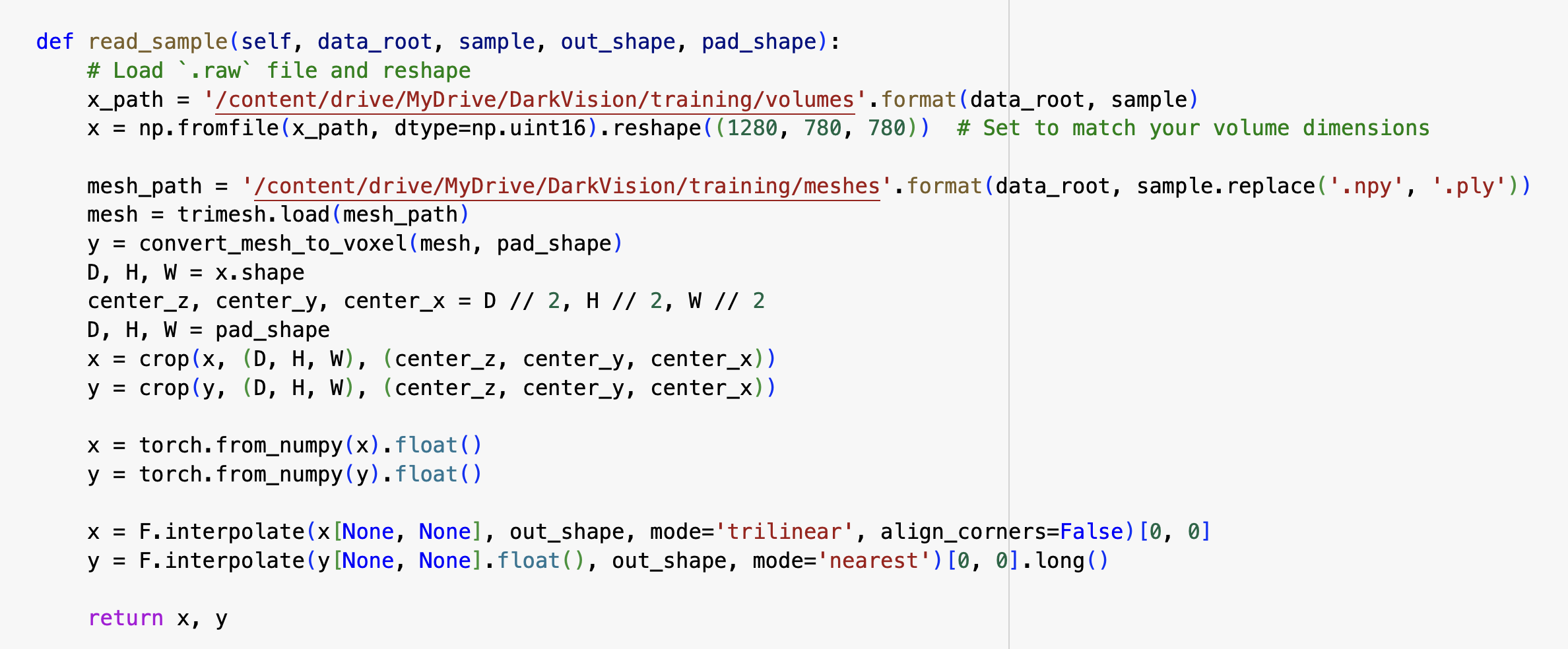
Above is our attempt in modifying the preprocessing section of the repository.
Reconstruction From Point Clouds
So when started out, we tried to generate the results using the author's model. We thought we succeeded at first (more on this later), so, we then attempted to make our own model. The repository has 4 files in order to build a desired model, as shown below:
- c0.py contains all of the distinctive parameters for the model itself, ranging from the number of recurrent layers to the number of epochs.
- c1args.py is where we preprocess the training data, both the ultrasound scans and the corresponding meshes.
- c2load.py is the core of the model. It requires all preceding files to be fully runnable in order to be executed.
- test.py is where the model is fed with the testing data and aims to reconstruct a surface mesh from given 3D volumetric data.
Model Architecture
Why did we choose the R2 U-Net model?
In all honesty, the R2 U-Net was one of the best performing models according to the paper, hence our decision. Additionally, this architecture was one of the three architectures that had most of the parameters defined from the authors comments within each separate file. Now let's get technical. As we know, residual layers allows us leverage skip connections, giving we have a deep layer; we wouldn't want the model to be unable to learn, countering the vanishing gradient problem. Other than that, recurrent layers are used so each convolution block would be able to learn from their past mistakes, feeding into the same convolution block for n amount of times.
In all honesty, the R2 U-Net was one of the best performing models according to the paper, hence our decision. Additionally, this architecture was one of the three architectures that had most of the parameters defined from the authors comments within each separate file. Now let's get technical. As we know, residual layers allows us leverage skip connections, giving we have a deep layer; we wouldn't want the model to be unable to learn, countering the vanishing gradient problem. Other than that, recurrent layers are used so each convolution block would be able to learn from their past mistakes, feeding into the same convolution block for n amount of times.
Results & Evaluation
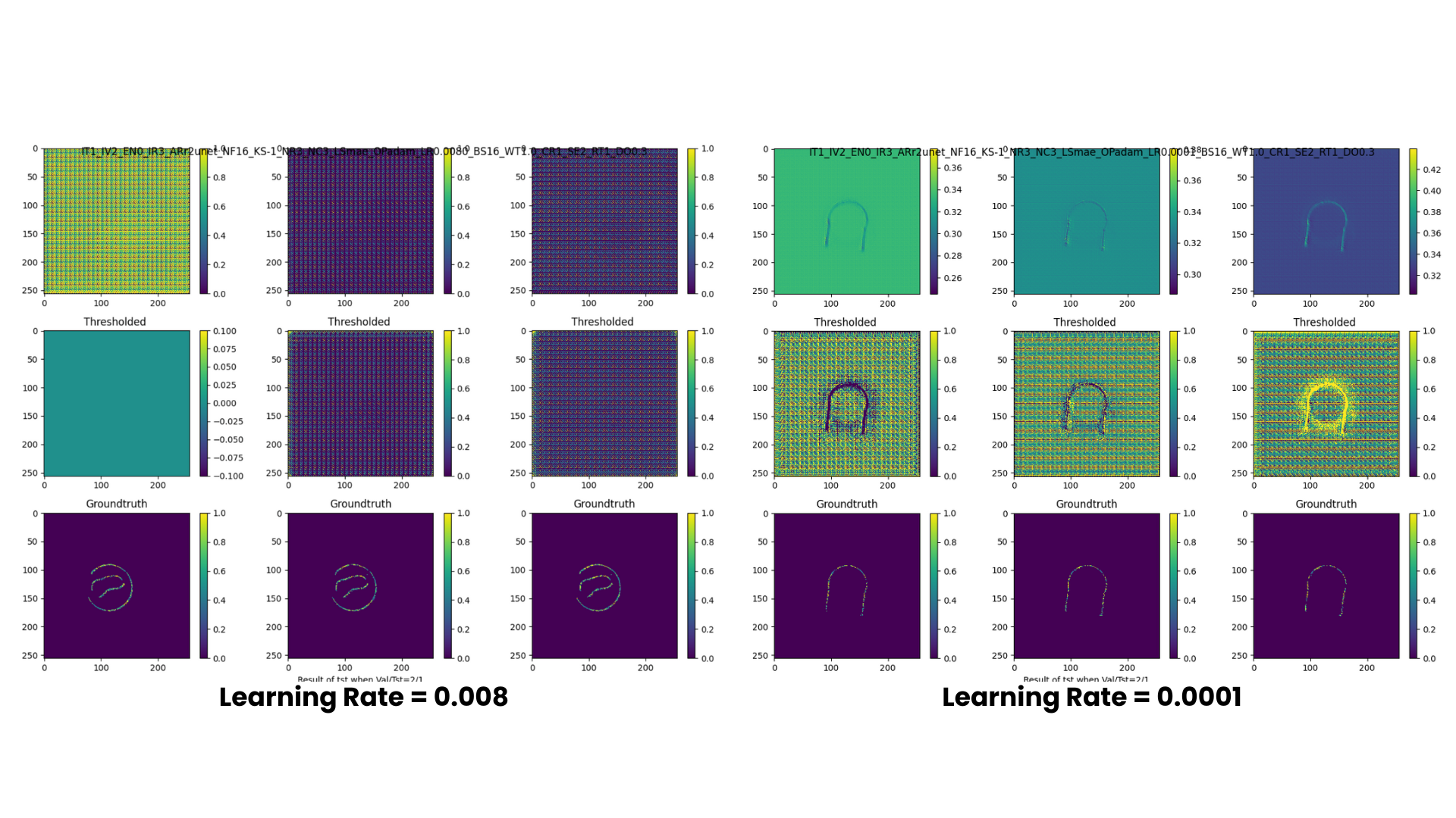
We were successful in generating our model in a .keras file format. Moreover, our model was able to read the training set as seen above. However, an anomaly worth pointing out is that fact that the readings seem to be inverted, meaning that what is read by the model to be the blank space is part of the steel pipe and vice versa. Additionally, we experimented different learning rates for our model. It is evident that 0.0001 yields a better reading.
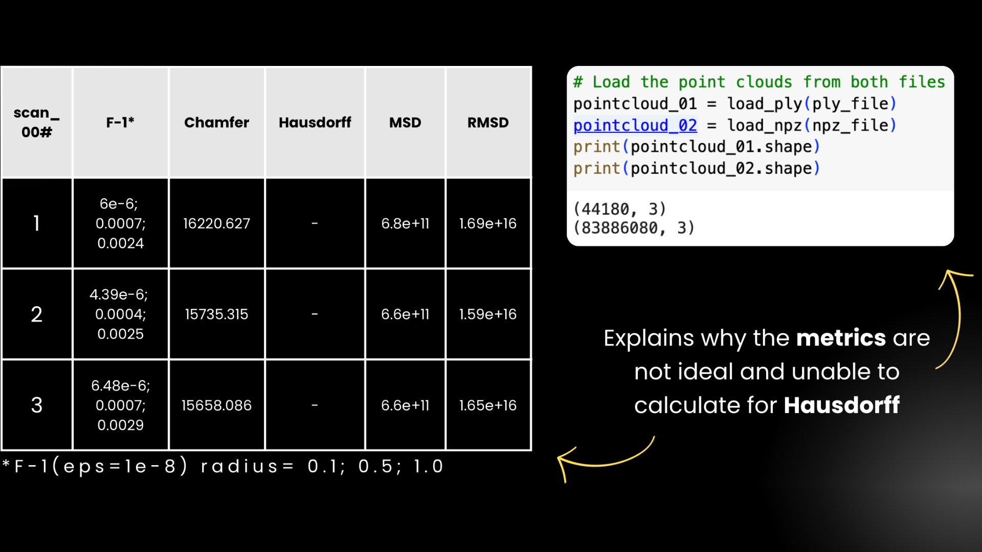
By using the model we saved earlier, we are inputting some of the steelpipe data, and then comparing it to the reference mesh by using 5 metrics:
- F1 Score: The harmonic mean of precision and recall, used to evaluate the performance of a classification model, especially in cases of imbalanced datasets. It is calculated as \(F1 = 2 \cdot \frac{\text{Precision} \cdot \text{Recall}}{\text{Precision} + \text{Recall}}\)
- Chamfer Distance: A metric used to measure the similarity between two point clouds. It computes the average minimum distance from each point in one point cloud to the nearest point in the other, and vice versa.
- Hausdorff Distance: A measure of similarity between two sets of points. It calculates the maximum distance from a point in one set to the closest point in the other set, considering all points in both sets.
- Mean Surface Distance (MSD): The average of the distances from points on one surface to the closest points on another surface. It provides a measure of how closely two surfaces align.
- Residual Mean Square Distance (RMSD): A measure of the average squared difference between the positions of corresponding points in two datasets, typically used in structural alignment or point cloud comparison. It is calculated as the square root of the average of squared differences between corresponding points.
For direct Hausdorff Distance values, we failed to calculate them because it took a very long time to run it. This is due to us having very limited time and resources, we decided to not include the values here. Along with us not able to calculate the Hausdorff Distance, we also see that the value for each metrics are not ideal for a functioning and viable model. We suspect that these problems are resulted due to the resulting npz file having so many points compared to the reference mesh. Here it says that the npz file contains 83 million points inside the array, compared to the mesh file which only has 40,000 points. This makes each metric produce a unreasonable value.
Challeges & Solutions
We breakdown our adversities into 4 categories: - Chronological Order: When we first looked at the repository, we didnt know which file was which and what their functions were, so we inspected each of the files and found out that there was a chronological order to the src code that allowed us to build our own model. - Untidiness and Lack of Comments: For example, when we tried to run our model in the test.py file, it gave an error telling us we had to have both the weights AND the model's architecture in our saved model. We traced back to our c2.py file, where the save_weights_only parameter was initially set to True. Hence, we changed it to False. However, it then gave us more problems for us to deal with which led to more debugging. - Undefined Objects: There were some objects present within files c1load.py and c2.py that were not previously defined. We resolved this through asking for more context to ChatGPT and Claude. It gave us a hint of intuition on how we were supposed to define these objects ourselves. - Outdated Code: We had to execute various pip install commands that were not listed on the demo notebook in order to run the metrics for our model.
Conclusion & Future Work
As we recall from the result, we can conclude that our model needs more work, as somehow it produced too many points. There was a reshape error that had to do with this part of the code. Here, we tried to visualize one of the resulting npz file of our model. It turned out to produced this 3D graph below, which has a ton of points. Not very much of a steel pipe right? This is more like a cube of points.
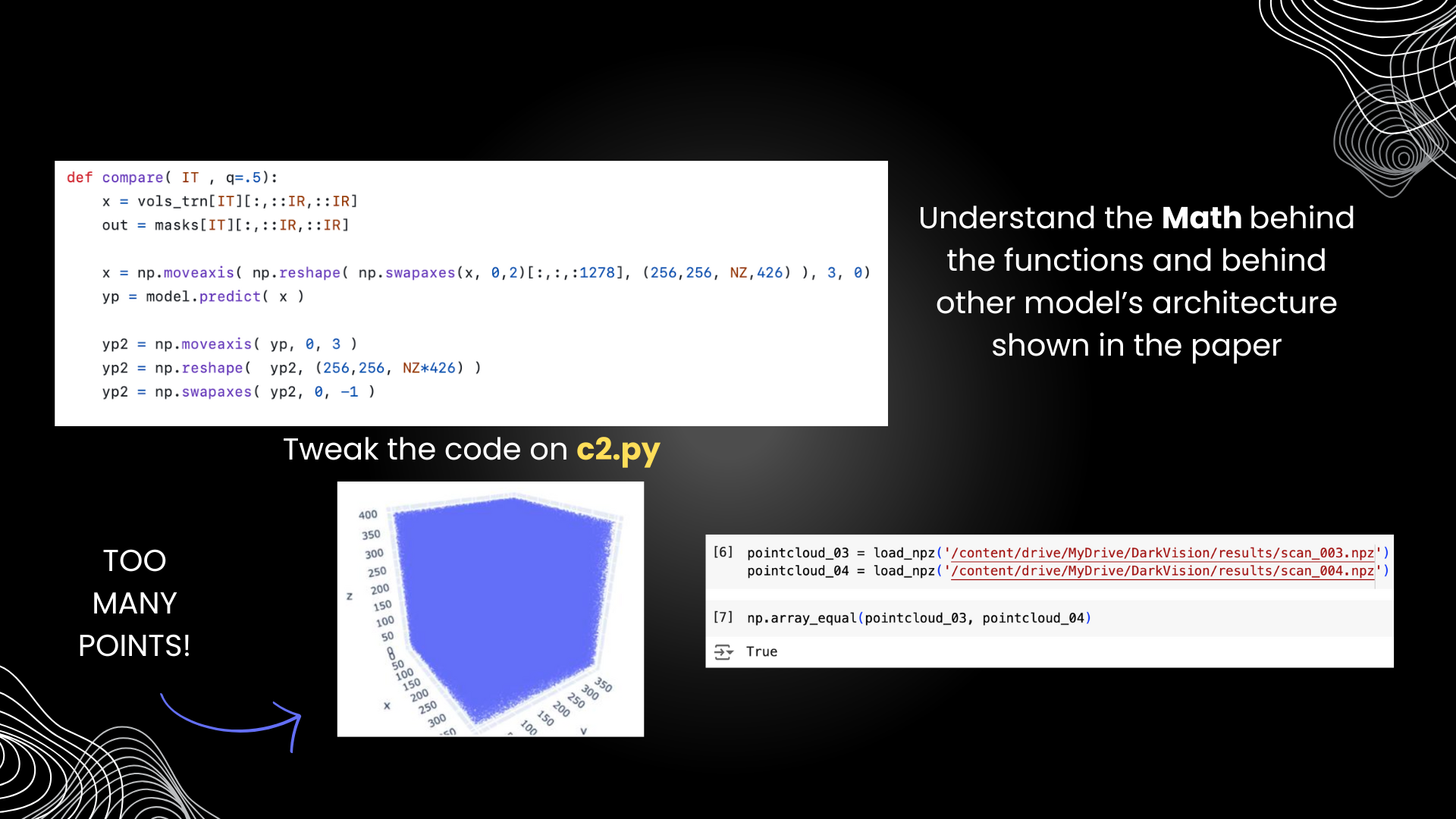
Then, we tried to investigate two different resulting npz files generated by our model, which was number 3 and 4. When we compared them using the np.array_equal function, it turned out to came out as true, even though they were produced from different inputs. This meant that our model was able to learn from the training model, as we presented earlier in the result section, but is unable to produce disntictive results.
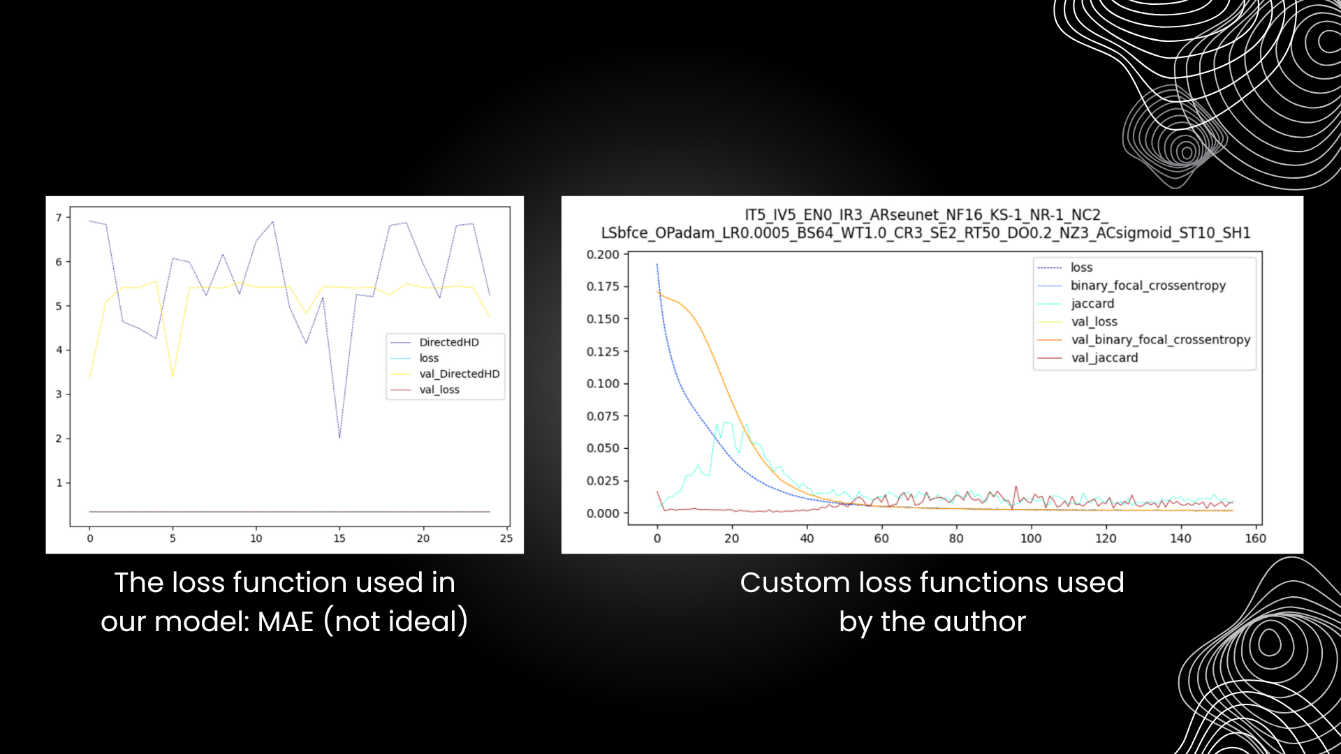
Furthermore, the metrics used to evaluate the model's performance was lacking compared to what the author presented in her paper. Future iterations should include proper metrics that are able assess the model's predictability better and show a decrease in the loss function. What we obtain (the left graph) wasn't an appropriate metric, as the variability shown clearly portrays its inability to assess our particular model, one that deals with 3D spatial data. Thank you for reading!
